Self-Organizing Maps

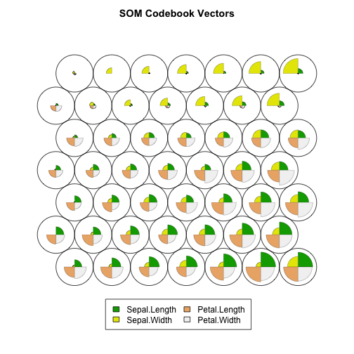
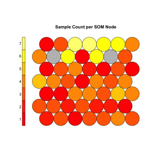
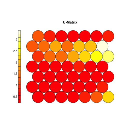
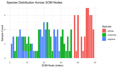
class: center, middle, inverse, title-slide

.title[
# Self-Organizing Maps
]
.subtitle[
## Kohonen Neural Networks for Data Visualization
]
.author[
### Mikhail Dozmorov
]
.institute[
### Virginia Commonwealth University
]
.date[
### 2025-12-01
]

---

<style>
.large { font-size: 130%; }
.small { font-size: 70%; }
.tiny { font-size: 40%; }
</style>

# What are Self-Organizing Maps?

- **Unsupervised neural network** technique invented by Teuvo Kohonen (1980s)

- Performs **dimensionality reduction** while preserving topology

- Maps high-dimensional data onto a low-dimensional grid (usually 2D)

- Key property: **similar inputs → nearby positions on map**

---
# Structure of a SOM

- **Input layer**: High-dimensional data vectors
  - Example: gene expression across 1,000 genes

- **Output layer**: 2D grid of neurons (e.g., 10×10 = 100 neurons)

- **Weight vectors**: Each neuron has weights matching input dimensionality
  - Each neuron represents a prototype in high-dimensional space

- **No hidden layers**: Direct mapping from input to output grid

---
# Training Algorithm: Overview

1. **Initialize** random weights for all grid neurons

2. **For each training sample**:
   - Find Best Matching Unit (BMU)
   - Update BMU and neighbors

3. **Repeat** for many iterations

4. **Result**: Self-organized topological map

---
# Training Step 1: Find BMU

- **Best Matching Unit (BMU)** = neuron closest to input

- Calculate distance between input vector and all neuron weights
  - Typically Euclidean distance

- Select neuron with minimum distance

```
distance = sqrt(sum((input - neuron_weights)^2))
```

---
# Training Step 2: Update Weights

- **Update BMU** to become more like the input

- **Update neighbors** based on distance from BMU

- Update formula:
```
new_weight = old_weight + learning_rate × neighborhood_function × (input - old_weight)
```

- **Neighborhood function**: Typically Gaussian, centered on BMU
  - Wide at start (many neighbors updated)
  - Narrows over time (only BMU updated at end)

---
# Key Properties

- **Topology preservation**: Adjacent neurons respond to similar inputs

- **Vector quantization**: Neurons become prototypes of input space

- **Competitive learning**: Neurons compete to represent each input

- **Self-organization**: Structure emerges from data, not imposed

---
# Gene Expression Example: Setup

**Scenario**: Analyze tumor samples based on gene expression

- **Samples**: 200 tumor biopsies

- **Features**: Expression levels of 5,000 genes per sample

- **Goal**: Identify molecular subtypes without predefined labels

---
# Gene Expression Example: Data

- **Input matrix**: 200 samples × 5,000 genes

- Each sample is a point in 5,000-dimensional space

- **Challenge**: Impossible to visualize directly

- **SOM solution**: Map onto 2D grid (e.g., 15×15)

---
# Gene Expression Example: Training

1. Initialize 15×15 grid (225 neurons)
   - Each neuron has 5,000 weights (one per gene)

2. Present tumor samples repeatedly

3. Neurons organize based on expression patterns

4. After training: similar tumors map to nearby grid positions

---
# Gene Expression Example: Results

**What emerges on the trained map**:

- **Clusters**: Groups of samples with similar expression
  - May correspond to tumor subtypes

- **Gradients**: Smooth transitions between subtypes

- **Outliers**: Isolated samples with unique profiles

---
# Gene Expression Example: Interpretation

**Analysis approaches**:

- **Component planes**: Visualize individual gene patterns across map
  - High expression genes for each region

- **Hit histogram**: Count samples per neuron
  - Identifies density of different subtypes

- **U-matrix**: Shows distances between neighboring neurons
  - Reveals cluster boundaries

---

# Gene Expression Example: Biological Insight

**Discovered patterns might reveal**:

- Aggressive vs. indolent tumor subtypes

- Response to specific therapies

- Activated biological pathways

- Novel biomarkers for classification

- Prognosis-related molecular signatures

---
## SOM example

---
## SOM example

---
## SOM example

<!---
# Applications Beyond Gene Expression

- **Customer segmentation**: Market research

- **Image analysis**: Texture classification, compression

- **Financial data**: Pattern recognition in time series

- **Quality control**: Process monitoring

- **Text mining**: Document organization

- **Robotics**: Sensor data analysis
-->

---
# Advantages

- Intuitive 2D visualization of complex data

- No assumptions about data distribution

- Preserves topological relationships

- Excellent for exploratory analysis

- Handles missing data reasonably well

- Interpretable component planes

---
# Limitations

- Grid size must be chosen beforehand
  - Too small: oversimplification
  - Too large: overfitting

- Computationally expensive for very large datasets

- Training can be slow

- Requires domain expertise for interpretation

- Modern alternatives (t-SNE, UMAP) often preferred for pure visualization

---
# Comparison with Other Methods

| Method | Supervised? | Preserves Topology? | Speed |
|--------|-------------|---------------------|-------|
| SOM | No | Yes | Moderate |
| PCA | No | No | Fast |
| t-SNE | No | Partially | Slow |
| UMAP | No | Partially | Fast |
| k-means | No | No | Fast |

---
# Implementation in R

``` r
library(kohonen)

# Prepare data matrix
data <- scale(gene_expression_matrix)

# Create SOM grid
som_grid <- somgrid(xdim = 15, ydim = 15, 
                    topo = "hexagonal")

# Train SOM
som_model <- som(data, grid = som_grid, 
                 rlen = 100, alpha = c(0.05, 0.01))
# Visualize
plot(som_model, type = "codes")
plot(som_model, type = "counts")
plot(som_model, type = "dist.neighbours")
```

---
## SOM on the iris Data

Use the numeric variables (150 samples × 4 features).

SOM performs better with **scaled** data.

``` r
library(kohonen)

# Extract numeric features
data(iris)
iris_mat <- as.matrix(scale(iris[, 1:4]))

dim(iris_mat)
```

```
## [1] 150   4
```

---
## Train the SOM Model

We use a **7×7 hexagonal grid**, which is good for small datasets.

``` r
som_grid <- somgrid(
  xdim = 7,
  ydim = 7,
  topo = "hexagonal"
)

set.seed(123)
som_model <- som(
  X = iris_mat,
  grid = som_grid,
  rlen = 200,
  alpha = c(0.05, 0.01)  # learning rate schedule
)
```

---
## SOM Codebook Vectors (Prototype Patterns)

Shows the “average pattern” for each neuron.

``` r
plot(som_model, type = "codes", main = "SOM Codebook Vectors")
```

![](SOM_files/figure-html/unnamed-chunk-7-1.png)

---
## Node Counts (Number of Samples In Each Cell)

This reveals cluster sizes and density.

``` r
plot(som_model, type = "counts", main = "Sample Count per SOM Node")
```

![](SOM_files/figure-html/unnamed-chunk-8-1.png)

Interpretation:

* Highly populated nodes = dense clusters
* Empty nodes = unused areas of the map

---
## U-Matrix (Neighbourhood Distances)

Visualizes distances between nodes — useful for clustering.

``` r
plot(som_model, type = "dist.neighbours", main = "U-Matrix")
```

![](SOM_files/figure-html/unnamed-chunk-9-1.png)

Interpretation:

* Light areas = similar neighboring units
* Dark borders = cluster boundaries

---
## Mapping Species to SOM Nodes

.pull-left[

``` r
# Assign each sample to its winning neuron
mapped <- som_model$unit.classif

df_map <- data.frame(
  Node = mapped,
  Species = iris$Species
)
```

Interpretation: If species cluster separately, SOM effectively discovered structure.
]
.pull-right[

``` r
library(ggplot2)

ggplot(df_map, aes(Node, fill = Species)) +
  geom_bar() +
  theme_minimal() +
  labs(title = "Species Distribution Across SOM Nodes",
       x = "SOM Node (index)",
       y = "Sample Count")
```

![](SOM_files/figure-html/unnamed-chunk-11-1.png)
]

---
# Key Takeaways

- SOMs reduce dimensionality while preserving data topology

- Self-organization emerges through competitive learning

- Excellent for exploring high-dimensional biological data

- Particularly useful when you don't know what patterns to expect

- Complements supervised methods for comprehensive analysis

---
# Resources

**R packages**:
- `kohonen`: Main SOM implementation
- `som`: Alternative implementation
- `popsom7`: A Fast, User-Friendly Implementation of Self-Organizing Maps

**Python packages**:
- `minisom`: Minimalistic SOM
- `somoclu`: GPU-accelerated SOM

.small[
https://CRAN.R-project.org/package=kohonen  
https://CRAN.R-project.org/package=som  
https://CRAN.R-project.org/package=popsom7  
https://pypi.org/project/MiniSom/  
https://pypi.org/project/somoclu/  
]

---
# References

- P. Tamayo, D. Slonim, J. Mesirov, Q. Zhu, S. Kitareewan, E. Dmitrovsky, E.S. Lander, & T.R. Golub, Interpreting patterns of gene expression with self-organizing maps: Methods and application to hematopoietic differentiation, Proc. Natl. Acad. Sci. U.S.A. 96 (6) 2907-2912, https://doi.org/10.1073/pnas.96.6.2907 (1999).

- Wehrens, R., & Kruisselbrink, J. (2018). Flexible Self-Organizing Maps in kohonen 3.0. Journal of Statistical Software, 87(7), 1–18. https://doi.org/10.18637/jss.v087.i07